UFood Marketing Data Analysis (Python)

Introduction

Welcome to my analysis of UFood's marketing activities, focusing on their marketing campaigns. UFood is a leading food delivery app, present in over a hundred cities. In the past three years, UFood has had solid revenues and a healthy bottom line, but the profit growth perspectives for the next three years are not promising. Because of this, the marketing team is looking for several strategic initiatives to reverse this situation.

The sample data provided consists of key customer information such as their income, age, marital and education status, amount spent on specific products and in total, and which of the five marketing campaigns (Six actually, we soon discovered a hidden campaign due to a data quality issue) they accepted.

Objective

This analysis enables UFood to increase campaign acceptance rate from 28% (current acceptance rate) to approximately 40% over the next three years, a 40% engagement increase achieved through data-driven targeting and personalized marketing strategies.

Stakeholder Questions:

1. How does age, marital status, household size, and education levels influence campaign responsiveness and total revenue contribution?

2. Which purchase method (Online, In-store, Catalog) should we prioritize marketing efforts on?

3. Can we define an "ideal customer" for targeted marketing?

The next portion of this report dives into cleaning and preparing the raw dataset to be useable. If you're more interested in the analysis and recommendations part, click here!

Also, click here if you want to see the full python code I created for this analysis.

Data Cleaning & Preparation

After importing the libraries we needed to conduct this analysis (Pandas, Matplotlib, Seaborn) and loading in the data, we begin by exploring the raw data to see if it needs to be cleaned and adjusted.

1. Dealing with Duplicates

We begin by checking to see if the dataset consists of any duplicates and assessing if they are a true duplicate.

Sample of duplicate data

Turns out, there are over 300 instances of duplicate records. While there is no unique customer ID that would help us confirm if these are true duplicates, I know that it's very unlikely that more than one customer can have the same exact income, age, education level, marital status, and spend the same amount on each product. Because of this, I can confidently say that these are true duplicates.

Now just because they're duplicate records doesn't mean it isn't good data to include in our analysis. These are likely real customers whose information was entered in more than once and because of this, we want to ensure that we keep only one instance of these records while deleting the rest.

By running this script, we drop every other instance of a duplicate record other than the first. The second line checks two distinct customers who originally had two instances of the same records, with the results showing that those customers now only have one instance of their records.

2. Combining Columns to Standardize the Data

   2.1. Total Children

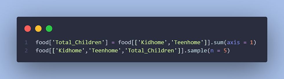
The original dataset had two distinct columns for those who had children; one for 'Kidhome' and one for 'Teenhome'. I wanted my household segmentation to be total children regardless of their age, so i combined these two into a Total_Children column.

2.2. Mapping the Marital Status

In the raw data, each customer originally has five separate binary columns containing either a 1 or 0 to indicate whether the customer falls into that specific marital status. To standardize this into one column, I assigned a unique numeric code to each status (5 for married, 4 for divorced, etc.), summed across the column to identify each person's marital status, and then map those values back to labels such as "Married" or "Divorced".

Before (Left) & After (Right), Same Customers

2.3. Mapping the Education Level

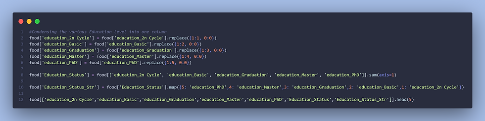
Similar to the marital status, we take the same approach to format the education level.

Before (Left) & After (Right), Same Customers

3. Finding Discrepancies in the Campaigns

Now by looking over the meta-data for this dataset, I found a key discrepancy. There are 5 campaigns listed, but another column labeled 'Response' is defined as '1 if customer accepted the offer in the last campaign, 0 otherwise'. This suggests that 'Response' should be treated as the sixth and final campaign indicator.

With this, I adjust an already-existing column within the dataset and create a new column:

1. The 'AcceptedCmpOverall' column calculated those who accepted campaigns 1-5. I now adjust it to count campaigns 1-6.

2. I create an 'Accepted_Campaign' that serves as a binary (yes/no) field for whether or not the customer accepted any campaign at all. If they did not, it will be 0. If they did, it will be 1 regardless of how many overall campaigns they accept.

Before (Top) & After (Bottom), Same Customers

4. Age Brackets

We finish the data cleaning and preparation by examining customer age and assigning the appropriate age bracket. To do this, we utilize a loop that checks each persons age and assigns them a label such as '31-40' or '41-50'. Grouping like this enhances the ability to segment and analyze behaviors such as likeliness to respond to a campaign or spending habits.

Analysis

Now that our data is cleaned and ready to use, I begin my analysis by using Python's corr() function with the Pearson method to analyze the relationship between various customer attributes with the binary variable Accepted_Campaign, which indicates whether a customer responded to any marketing campaign. Doing this allows us to identify which features are most strongly associated with campaign responsiveness.

Based on these results, we can draw some key initial insights (Needs further investigation):

1. A high correlation with 'AcceptedCmpOverall' suggests that customers who sign up for one campaign are very likely to sign up for multiple.

2. Wine purchases (MntWines) have the strongest product-spending correlation (~.42), followed by meat purchases (MntMeatProducts).

3. Negative correlations with Teenhome (~.13), Kidhome (~.18), and Total_Children (~.22) suggests customers with more children tend to accept fewer campaigns.

Next, I want to use the Seaborn and Matplotlib libraries to generate a point plot that visualizes how campaign acceptance varies across predefined age groups.

Now within this visual, the vertical lines represent the confidence intervals. What this visual tells me is that age groups 23-30 and 71-85 may accept campaigns at a higher rate than the other age groups, however there is probably a small sample size of these age groups.

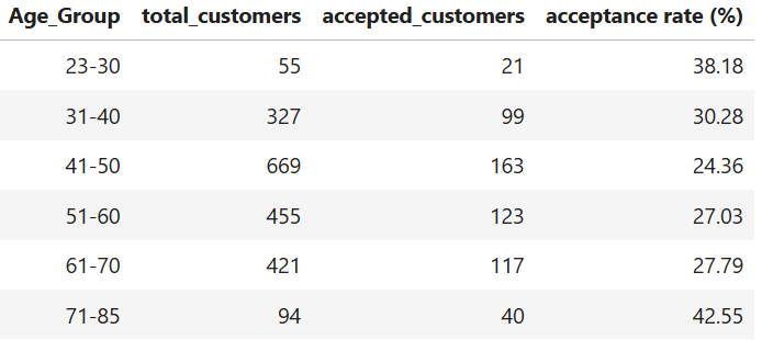
And my hypothesis was correct; age groups 23-30 and 71+ have the highest campaign acceptance rates while having the smallest customer base. The majority of customers sit between ages 31-70. Something to keep in mind for later as we move on with the analysis.

Now while still focusing on accepted campaigns, I want to compare both total and campaign-specific spending across age groups. I do this by creating two result sets: Total_Spending and Result_Spending. I then use the melt function to pivot the data into one DataFrame, making it easier to visualize spending types side by side.

Now we see how much each age groups spends in total and when a campaign is accepted. As we may have expected, those between the ages of 31-70 (who represent over 90% of our customer base) generate the majority of revenue. In our final recommendations, I outline an in-depth strategy to capitalize on profit and campaign acceptances based on these findings.

Now to further identify which customers to target for future campaigns, we first need to determine where campaign acceptance is occurring most often. At the customer level, our dataset provides counts of purchases made through three main channels: catalog (NumCatalogPurchases), in-store (NumStorePurchases), and online via the company website (NumWebPurchases).

Let's visualize this to see where the bulk of our overall traffic comes from as well as how effective campaigns are at each channel.

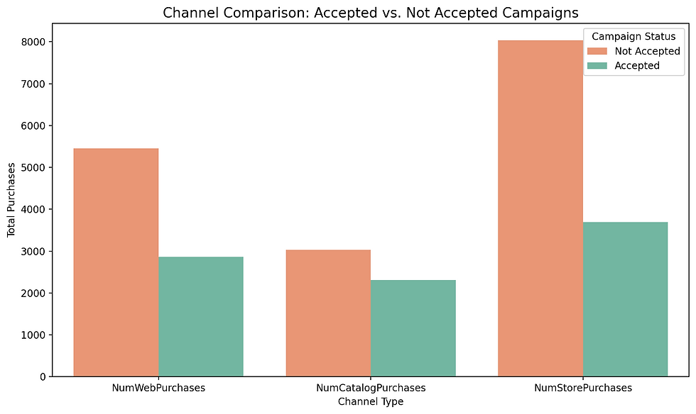
We visually see that while in-store and online purchases drive more overall traffic, catalog purchases yield higher conversions among customers who accept campaigns.

I now want to see how the amount of children within the customer household impacts spending and campaign acceptance. To do so, we'll create regression plots that analyze how the number of children relates to customer behavior.

Here we see a negative correlation between total children and customer behavior, suggesting that as the household grows, customers may be less responsive to campaigns and overall spending.

Now let's take this same approach but look at how education level compares to customer behavior.

Unlike the amount of children within a customers household, education level shows only a slight positive correlation with campaign acceptance and overall spending, however the relationship appears weak and not statistically significant enough to serve as a predictor for campaign targeting.

Now we wrap up our analysis by comparing customer spending by their marital status, by overall spending as well as when they accepted a campaign.

This visualization shows that Married, Single, and Together customers are the strongest candidates for future campaign targeting. I decided to display these results as two separate bar plots rather than a side by side one to uncover a notable discrepancy: although customers in the Together group spent more overall than those who were Single, it was the Single customers who contributed slightly more spending when they accepted a campaign. This suggests that they may be more responsive to targeted offers.

Final Recommendations

Now that I've run the analysis and better understood our customer base, I'm excited to present these insights and recommendations to the marketing team.

1. Age Group Segmentation

The point plot and bar plot that I created showed that those between the ages of 31-70 made up a majority (90%+) of our customer base and therefore drove in most of our revenue, even through a campaign. However, age groups 23-30 and those 71 and up, who represented a small portion of our sample, were accepting campaigns at a higher rate. This leads to a couple ways we can strategize a boost in campaign hit rates:

• Strategy 1: Prioritize Core Segments (31-70)

  Focus on strengthening engagement with our largest customer group by personalizing campaigns around their preferences and behaviors.

• Strategy 2: Cultivating Engagement with Outliers (23-30, 71+)

Despite their smaller size, these groups demonstrate a strong receptiveness to campaigns. We can capitalize on this by investing in targeted acquisition and retention strategies (onboarding incentives, referral programs, and tailored messaging) to grow the customer base as a whole and their value over time.

2. Purchase Type Comparison

The majority of purchases made by customers seem to be from in-store and through the online site. With that said, catalog purchases yielded higher conversions among customers who accept campaigns. I would recommend a split between all:

• 40% catalog, 30% online, 30% in-store (Monitor ROI across segments and make adjustments based on lift performance in year 1).

3. Household Segmentation

The regression plots I created showed a negative correlation between total children and total spent as well as when it came to accepting campaigns. This would suggest prioritizing customers with fewer or no children as they would be more likely to spend more money and accept a campaign, making them a stronger target for future marketing efforts.

4. Education-Level Segmentation

When we recreated the same type of analysis for the various education levels, we saw minimal impact. While there is a slight positive correlation as education level rises, it didn't seem significant enough to say that those with higher education levels are more likely to accept a campaign.

5. Marital Status Segmentation

Customers within the Married, Single, and Together status are the strongest candidates for future campaign targeting. Single customer specifically stand out for their higher campaign-driven spending when compared to customer within the Together status, indicating a strong responsiveness to targeted offers despite spending spending less outside of campaigns.

6. Ideal Customer Profile

Based on my analysis, the ICP (Ideal Customer Profile) would be someone who is single, aged 41-50, has few or no children, and often purchase through the catalog channel. Additionally, the use of the correlation function early in the analysis showed elevated spending specifically on wine and meat products.

• Using SQL for calculations, I found that customers who were single, between ages 41 to 50, and had 1 or no child had an underwhelming 28% acceptance rate to campaigns. Getting this up to a 60% acceptance rate would be a good place to start to boost overall engagement.

Final Thoughts

This project opened my eyes to the depth of insights that can be drawn from a marketing-focused dataset. The ability to group, segment, and visualize customer attributes revealed insightful behavioral patterns that can shape real-world marketing campaign strategies.

As I continue to deepen my Python skills, I can see myself coming back to this analysis and expanding on it. I am particularly interested in learning techniques like K-Means Clustering and Predictive Modeling to really expand on this analysis.

I want to thank Alex Fredberg for his guidance on this project and for teaching me such a complex language from the ground up as well as the Python community on Stack Overflow for code support and troubleshooting.